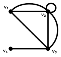
In many cases and situations, we need to represent a graph in the form of mathematical equations or formulas, as this will help us analyse the graph easier. Before we learn how to use a matrix to represent a graph, we’ll first consider representing a graph in a list. We call it an adjacency list. By the way, the word ‘adjacent’ means ‘next to’. This list shows us the vertices, and its adjacent vertices and how they are related. For example, the graph below is represented by its adjacency list on the right.
Notice that some adjacent vertices are double counted due to multiple edges. You should be able to create an adjacency list from a given graph, and also sketch the graph with a given adjacency list.
The above adjacency list was for an undirected graph. An adjacency list for a directed graph looks like the one below:
Sometimes it really doesn’t matter whether you have dots or circles. Notice that this adjacency list has its top row labelled with the initial and terminal vertices, which differs from the previous one.
As you know, anything that can be represented in a table can be represented in a matrix. There are 2 kinds of matrices that we can represent a graph with:
1. Adjacency Matrix
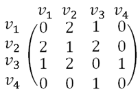
Consider the graph above. Once we label down all the vertices, we can represent it as an adjacency matrix, with the rows and columns being the vertices. When there is an edge connecting 2 vertices v1 and v2, then the slot in the matrix will show the number 1, and if there are 2 edges, then it will be 2, and vice versa. Note that if there exist a loop in a vertex itself, it only counts as 1 edge, unlike the degree of vertex when we counted 2. The adjacency matrix of the graph above is like the one below.
You don’t really need to label the vertices in the matrix, I put it there for clarity. An adjacency matrix for a directed graph is slightly different. The rows represent the initial vertices, while the columns represent the terminal vertices. Take a look at the graph and its adjacency matrix below:
This matrix is the more useful one. It helps us to find the number of paths with a certain length between a pair of vertices. The power of the matrix Mn represents the length of a path. So if we square the matrix above, getting
gives us a new matrix which shows us the amount of paths with length 2 from vertex to another. It means, there is 1 path of length 2 from a to a, 3 paths of length 2 from b to a and etc. When I find M3, it will be paths of length 3 and so on. With this, we are able to find the shortest path for one vertex to reach another vertex and also to find the number of paths of a particular length from one vertex to another. In cases where you have graph of vertices more than 4 or 5, you may want to consider multiplying the particular row and column only to find the required answer, as evaluating the whole matrix will be wasting your time.
One more thing to note, is that the sum of a row is not the degree of vertex for a pseudograph, since the count of loops will be wrong. You need to double count the loops in order to get the correct degree of vertex.
2. Incident Matrix
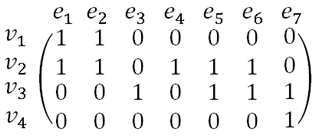
To create an incident matrix, you need to label all the edges as well. For this matrix, the rows are the vertices, but the columns are the edges. So for every slot in the matrix, it will be 1 if its vertex is connected to that edge and 0 if none of the above. See the graph above, and its incident matrix below:
Multiplying this matrix with itself won’t get you anywhere. Notice that every column adds up to 2, except if it is a loop. This is because, every edge is connected to 2 vertices. Again similar to the adjacency matrix, adding up the rows will not give you the degree of vertex if it is a pseudograph.
PROBLEM MODELLING
Graph theory has many uses, as it can help us solve some complicated, as well as some simple daily problems. In planning for a flight route, you could construct a graph where the vertices are places, edges exist when there is a flight between the two places. In an assignment of a team to do a particular project, we can use graphs to assign who to do what, after knowing the abilities and talents of the individuals.
Some examples of graph models:
Acquaintance graphs:
Vertices represent people. ab is an edge if a and b know each other.
Influence graphs:
In studies of group behaviour, it is observed that certain people can influence the thinking of others. A digraph can be used to model this: uv is a directed edge if u can influence v.
Call graphs:
Directed multigraphs can be used to model telephone calls in a network. Here telephones are represented as vertices and each call from a to b is represented by ab. From this graph, we can actually deduce who has changed his phone number by viewing who the new phone line contacts, and who has not used his phone for a long while.
Web graphs: The World Wide Web can be modelled as a digraph where each webpage is represented by a vertex. There is a directed edge ab is there is a link on a pointing to b.
Precedence graph:
Computer programs can be executed more rapidly by executing certain statements concurrently. However, certain statements depends on the results from other statements. Thus we to create a precedence graphs. Here each vertex represents a statement. A directed edge ab means that a must be executed before b.
Dual graph:
The resulting graph of a map. You represent a map with a graph. For example,
The red graph G’ is the dual graph of the existing graph G. The red dots represent a region, and an edge exists between two vertices when the regions are adjacent to each other.
A more interesting one is the weighted graph, which is a graph that has a number assigned to each edge. These numbers could represent the distance between 2 cities, the airfare between 2 cities, and we could actually come out with a shortest / cheapest path from a place to the other. Let me give you an example:
Let’s say, the alphabets A to G all represent a name of a place, and the numbers represent the time (minutes) to get to each town by car. We want to find the path which takes the shortest time to get from town A to town G. To do this, we will make use of Dijkstra’s Algorithm. I won’t explain this algorithm in words (as even I don’t understand what the textbook talks about), but I’ll briefly show you how it’s done.
Starting from A, you find the shortest edge to its adjacent town. It is D, which takes 2 minutes. Then find the shortest time to reach B, and we see that it takes 7 minutes. Now, all the adjacent towns of A are done, we shall proceed to the adjacent towns to D and B, which are C, E and F. From A, the shortest distance to F, you get there either by passing B or D, don’t you? And obviously, you make use of the route with the shortest time to both of those towns. So make use of those 2 routes, we find that the shortest time to F is 11 minutes (ADF). We further find that the shortest time to E and C are 14 minutes (ABE) and 15 minutes (ABC) respectively. Using these 3 routes, we find the shortest time to get to G, which is obviously, the ADFG route, 22 minutes.
Try googling for the Travelling Salesman Problem. It has something related to this issue over here.
There is no easy way to solve these problems, as things will become quite complicated if the number of vertices and edges are large. I suggest once you found a solution for this kind of questions, leave it as it is first. After you finished the paper, come back to this question, and triple check whether there is any other shorter routes. Do lots of practices. ☺


No comments:
Post a Comment