Pages

Monday, May 30, 2011

2.1 – Polar Form

The basics of this chapter on complex numbers should have been covered in Mathematics T. So while I explain stuff over here, I assume that you already know the following about complex numbers:

a. understand what is the real part, imaginary part, and conjugate of a complex number
b. find the modulus and argument of a complex number
c. represent complex numbers geometrically by means of an Argand diagram
d. use the condition for the equality of two complex numbers
e. carry out elementary operations on complex numbers expressed in
Cartesian form

So in this post, I’ll be introducing to you another 2 forms of which you can represent a complex number. This will be a short one.


You still remember that the modulus of a complex number, a + bi is denoted by |z|, which has the value √(a2 + b2). And then, you also remember that the argument of a complex number, denoted by arg z, has the value of tan-1 (b / a), putting in account which quadrant is the complex number in the Argand diagram. So with the modulus and argument, you can represent a complex number in polar form, or (r, θ) form, which is

|z| (cos (arg z) + i sin (arg z))

For example, the modulus of the complex number –3 + 3i is 3√2, its argument is 3π/4, so its polar form is 3√2 [ cos (3π/4) + i sin (3π/4)]. Using this form will give us a lot of advantages, especially when we learn de Moivre’s theorem in the next post.

Another way of expressing complex numbers using the argument and modulus is the exponential form. The term cos θ + i sin θ can be written as e, where e is the natural exponent. So by multiplying the modulus in the front of both terms, and substituting the θ with the argument, you get another form of complex numbers! Using the example above, the exponential form of –3 + 3i is 3√2ei(3π/4).
This is something like a compressed form of complex numbers. By now you will be puzzled as in how do you relate cosine and sine with exponents. Well, I’ll show the derivation, only in the chapter Power Series. As for now, just take it as it is. (Extra info: go google for “Euler’s Equation”. You will be surprised by the equation e+ 1 = 0 !)


Now that we know 2 extra forms of complex numbers, we want to know how multiplication and division of complex numbers can be done easily in these 2 forms. The general rule is this:
When you multiply 2 complex numbers, you multiply their modulus and add up their arguments. But when you divide 2 complex numbers, you divide their modulus and subtract their arguments.

Let’s give it a try. Suppose we multiply 2 complex numbers, –3 + 3i and –1 – i. You will have:
3√2 [ cos (3π/4) + i sin (3π/4)] × √2 [ cos (3π/4) - i sin (3π/4)] = 6
Did you catch my working? Try using some trigonometry formulas, you will eventually get the answer. Take note that 3π/4 - 3π/4 = 0!
There’s also another way of going about it. Let’s try using the exponential form:
3√2ei(3π/4) × √2ei(-3π/4) = 6

This is multiplication. It will be the same for division, go ahead and give it a try. There’s no shortcut for addition and subtraction though, so it’s better to use the cartesian form to solve them.


Now we will learn the geometrical effects of basic operations on complex numbers. We will be using the Argand diagram (which I assume you already know what it is, and what are its axes).

1. Conjugation
image
Basically what conjugation does is that it reflects a complex number across the real axis. Try visualizing these complex numbers as vectors, and you will understand more.

2.
Addition & Subtraction
image
The diagram above shows the addition of 1 + 1i with 1 – 1i. As you can see, it is merely a vector addition, you add up the two of the complex numbers as if they were vectors. You should be able to deduce that for subtraction, just by using the fact that the added minus sign switches the direction of the arrow, you will be able to get the answer, which will be 2i, lying on the imaginary axis. Quite straightforward right?

3.
Multiplication & Division
image
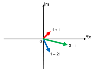
Possibly you couldn’t catch what the diagram meant. The green arrow, 3 – i is the result of the multiplication of 1 + i and 1 – 2i. What happens here is just exactly what we learnt above: the modulus multiplies (the length does not add up, but multiplies as in √2 × √5 = √10) and the argument adds up (0.25π rad – 0.35π rad = –0.1π rad). You can try expressing the complex numbers in polar form, which will help you to identify it clearer. These are really simple stuff, because your head will start to spin when the loci of complex numbers come in.


That’s all for this section. Do more exercises on converting complex numbers from the Cartesian form to the polar form. We’ll proceed to unleashing the power of de Moivre’s theorem on the polar form of complex numbers!

Sunday, May 29, 2011

1.2 – Proof

A theorem is a statement that can be shown true.
A proof  is a valid argument that establishes the truth of a theorem.

In this section, I will be showing you 3 main kinds of proof (with tonnes of sub-proofs).


DIRECT PROOF

This proof is very straightforward. A direct proof  of a conditional statement pq, is shown by showing that p is true, then show that q is true. Basically what it means is that you show that something is true, and therefore some other thing follows to be true as well. Let me give you an example:

Show that the sum of 2 odd integers is even.

Did you notice that this is actually a conditional statement? We let p be ‘m & n are odd integers’ and q be ‘the sum of m & n are even’. Putting pq, we have ‘If m & n are odd, then their sum is even’. So the proof is:

Let m = 2j + 1, and n = 2k + 1, where j and k are integers. Here we can see that m & n are odd. Then m + n = (2j + 1) + (2k + 1) = 2(j+k+1), which is even.
Therefore, the statement is proven valid.

Try to get used to the definition of odd and even integers, being 2k + 1 and 2k respectively, where k is an arbitrary integer (arbitrary means ‘anything’). Actually, when you are asked to prove odd and even integer stuff, it will definitely be a direct proof, and just substitute these definitions in, then you will find the answer. Another case is in proving theorems related to perfect squares, where you use the definition n = k2. One more case is in proving rational and irrational numbers, where you define a rational number n = j/k. All these definitions will help you a lot, and you may use it in the later chapters, like Number Theory


INDIRECT PROOF

Literally, an indirect proof is a proof that is not direct, i.e. you don’t prove straight using pq. There are many kinds of indirect proofs:

1. Proof by Contraposition
This proof basically proves the statement pq using its contrapositive, which is ~q~p. Example:

Show that if x + y ≥ 2 (where x & y ϵ R), then x ≥ 1 or y ≥ 1.

Looking at the question, you know you won’t get anywhere if you try to manipulate the first statement, x + y ≥ 2. So what you do is by assuming that ~q is true, which means x < 1 and y < 1. Remember the fact that the contrapositive of a conditional statement has the same truth value as it has! So here we have

Suppose x < 1 and y < 1. Then x + y < 1 + 1, x + y < 2, which is the negation of x + y ≥ 2. Therefore, the statement is proven valid.

2. Proof by Contradiction (Reductio ad absurdum)
What this proof does is to first assume that p is true, and ~q is true (p→~q). You will eventually evaluate ~q and find out that ~p is also true. Now you have p Λ ~p, which is a contradiction (a statement which is always false)! From here, you conclude that pq. Example:

Prove that the sum of an irrational number and a rational number is irrational.

Putting it in a pq form, we rewrite the statement as ‘if m & n are irrational and rational respectively, then their sum is not rational’. Now let’s try solving it:

Suppose r is rational and i is irrational, and r + i = s is rational.  [p is true, ~q is true]
Then s could be written as p/q for some integers p and q which have no common factors. r could also be written in the form t/u, where t and u are integers with no common factors too. Using some algebra,
image
which is contradicting, since i is irrational. So it follows that the sum of an irrational number and a rational number is irrational.

3. Vacuous Proof
All you need to do in this proof is to show that p in the pq statement is false. (Note that when p is false, the statement will definitely be false!) This is used to proof statements like ‘if 2 + 2 = 5, then it will snow in Malaysia’. Won’t come out in STPM, I assume…

4. Trivial Proof
This proof is similar to the above, but here you must show that q is true in the pq statement. (Once again recall, when q is true, whether p is true or false, the statement still holds!) For the statement ‘if you give me RM1, then the sun will rise in the east’. I don’t need to explain, right?

5. Proof of Equivalence
This proof is for proving statements of the form pq, where you need to prove pq and its converse, qp. You can use one of the above methods (direct proof, proof by contraposition or contradiction) to solve the pq and qp part. Basically this proof is a combination of proofs, and I don’t think I need to elaborate much on this.

6. Proof by Cases
In this proof, you need to proof something using a case by case basis. For example, Prove that |x| + 2 > 0.
I won’t show you the answer. All you need to do is use case by case: case 1 where x > 0, case 2 where x < 0, and case 3 where x = 0, substitute the values of x in it, then show that it is true.

7. Exhaustive Proof
This proof requires you to use up all the possibly numbers in that domain, substitute them into the equation to show that it is valid. E.g.,
Prove that n2 + 1 > 2n, where 0 < n < 5. Just use up all the values n = 1, 2, 3, 4 and substitute them into the equation to prove it. Very straightforward for a small domain of n.

8. Existence Proof
The questions for this kind of proof normally starts with something like ‘show that there exist a…’. There are 2 kinds of existence proof, it can either be constructive or non-constructive. A constructive one will make you find the exact answer to the question, while the non-constructive approach will prove the statement true even without finding a solution. I’ll show you the examples:

Show that there is an integer that can written as the sum of cubes of two integers in two different ways.
This is true as 1729 = 103 + 93 = 123 + 13.
[constructive]

Show that the equation x3 + x - 1 = 0 has a solution.
Let P(x) = x3 + x - 1. Then P(0) = -1 and P(1) = 1. Thus (by the intermediate value theorem), the equation P(x) = 0 has a solution which is between 0 and 1.
[non-constructive. Interesting isn’t it?]

9. Uniqueness Proof
This proof is an extension of the previous proof. First you show that there is a solution x for the statement P(x). Then you find a value of c which is true for P(x). So lastly, you show that if x ≠ c, then
P(x) is false. Example:

Show that if a, b ϵ R with a ≠ 0, there is unique r ϵ R such that ar - b = 0.
Certainly r = b/a satisfies ar - b = 0. [1st & 2nd part]
Next, suppose s, t both satisfy as - b = 0 and at - b = 0. Then as - b = at - b and so as = at. Since a ≠ 0, we have s = t, which means that the solution is unique.
[3rd part]

10. Proof by giving a Counterexample
A counterexample is used to disprove something. This is super easy, for example:

Prove or disprove that the product of 2 irrational numbers is irrational.
Using a counterexample, √2 × √2 = 2, which is rational. So the statement is invalid.

All you need to disprove something is to find a counterexample. That’s it.


MATHEMATICAL INDUCTION

Mathematical induction
is the most common proof that you will use and see in your exams. There are lots of information on this proof in A-level books, so I don’t need to give you too much examples. What mathematical induction does is that it proves that an equation is true for a particular value, we call it the basis. Then we go on to prove that the equation is valid for any value greater than that basis. To sum up, mathematical induction involves 2 steps:

1. The basis step: you proof that the equation is true for n = 0, n = 1 or whatever initial value they give you in the question.
2. The inductive step: you now assume that the equation is true for n = k. Then you try solving the equation in terms of n = k + 1, and show that the relationship holds too. From here you can conclude that by mathematical induction, the equation is true in that domain.

Let me show you an example:

Use proof by induction to prove that
image

Since
image
LHS = RHS, we see that the formula is true for n = 1. We assume that the formula is true for n = k, then we have

image
and letting n = k+1, we have
image

Hence
image
is true for all n ≥ 1. [proven]

I will show you some tips on how to solve different kinds of questions. Remember to do A LOT of exercises on Mathematical Induction!

* Questions involving summations
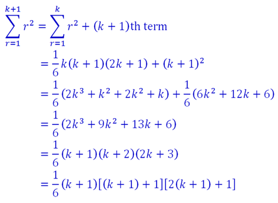
Try to make use of the fact
image

* Questions involving matrices
Try to make use of the fact
Ak+1 = Ak × A, where A is a matrix.

* Questions involving differentials
Try to make use of the fact
image

* Questions involving recurring terms
Try to make use of the fact
if un + un+1 is divisible by a, then either un & un+1 are both divisible by a, or both not divisible by a.


That’s all for chapter 1. For this section, focus more on mathematical induction, direct proofs and proof by contraposition.

Friday, May 27, 2011

1.1 – Logic

A proposition is a declarative sentence that is either true or false, but not both. Normally, we will use the letters p, q and r to represent a proposition. The negation of a proposition is its opposite. For example, if p: 2 + 3 = 5, then its negation is 2 + 3 ≠ 5. A negation of p can be represented by ~p, or ¬p. It is recommended that you stick to one, so I will be using ~p throughout this post.


Given 2 propositions p and q, a conjunction has the meaning of 'p and q'. Symbolically, it can be written as pq.

A disjunction has the meaning of 'p or q'. Symbolically, it can be written as pq. There are some other disjunctions which we don’t normally use, like the 'exclusive or' (pq), 'not and' (nand, p | q) and 'nor' (pq).

An implication is a conditional statement, where p is the antecedent (hypothesis or premise) while q is the consequence (or conclusion). It has the meaning ‘if p, then q’. Symbolically, it can be written as pq. In English, there are many ways you can interpret this other than ‘if p, then q’. Examples are

  • If p, q.
  • q unless not p.
  • p implies q.
  • p is sufficient for q.
  • p only if q.
  • q when p.
  • q if p.
  • q whatever p.
  • A necessary condition of p is q.
  • A sufficient condition of q is p.
  • q is necessary for p.
  • q follows from p.

A bi-implication is a bi-conditional statement, which means that the implication and its converse are equivalent. It has the meaning ‘p if and only if q’. Symbolically, it can be written as pq. Other ways of saying it are

  • p is necessary and sufficient for q.
  • If p then q, and conversely.
  • p iff q.

Now using a conditional statement pq,

  • A converse of the statement is qp.
  • An inverse of the statement is ~p → ~q.
  • A contrapositive of the statement is ~q → ~p.

To further elaborate the meanings of all the stuff above, I’ll continue by introducing truth tables.


TRUTH TABLES

A truth table is a table which states the truth values of various statements. Here, ‘T’ means ‘true’, while ‘F’ means ‘false’. So the truth table for negation is

 p   p̅ 
T F
F T

which means that every time when p is true, is false and whenever p is false, is true.

Let’s go on for conjunctions, disjunctions, implications and bi-implications:

 p   q   p  q   p  q    q    q 
T T T T T T
T F F T F F
F T F T T F
F F F F T T

Summarising the results above,

  • pq is true if both p and q are true;
  • pq is true if either one of p or q is true;
  • pq is true if both p and q are true, or both p and q are false;
  • pq is a little tricky: it is only false when p is true and q is false.

To further understand the results of pq, let's use an illustration. Suppose a certain political party in Malaysia gives a conditional statement: “If we win the next elections, we will immediately reduce the price of petrol by 20%.” So according to their statement, there will be two outcomes:

Situation 1: They won the elections
In the event that they really did reduce the petrol price, then the statement is true. But if they break their promise and the petrol price isn’t reduced, then the statement is false.

Situation 2: They lost the elections
Since they didn’t promise anything about what they will do if they lost, whatever that happens, be it the price of petrol increases, remains or reduces, doesn’t make the statement false, and so therefore, for either case, the statement is true.

Now we’ll go on to see the truth tables for converse, inverse and contrapositive:

 p 
 
 q 
 
 p  q 
 
 q  p
 (Converse)  
 ~ ~q 
 (Inverse) 
 ~q  ~p 
 (Contrapositive) 
T T T T T T
T F F T T F
F T T F F T
F F T T T T

Notice that the converse is equivalent to the inverse! Besides, the statement itself is equivalent to its contrapositive. This is a very important piece of information when studying logic.


PRECEDENCE

In problem solving, you can combine all the logical operators to make a very complicated statement. For example, you can have
[ (~r ∧ ~p) q ] ∧ [ q (~r ∨ ~p) ]

In order to understand the statement, you need to have a precedence of logical operators, which means, which symbol comes first and which comes second and so on. The precedence of logical operators, from first to last is as follows: ~, ∧,∨,→,↔.


If 2 statements have the same truth values, we say that the statements are logically equivalent. if p and q are logically equivalent, we write p ≡ q. Note that it is an equal sign with 3 strokes instead of 2.

A tautology is a compound proposition that is always true, no matter what the truth values of the propositions that occur in. For example, ~p (p q) is a tautology. You can check by looking at its truth table below:
image

Opposite to a tautology is a contradiction, a compound proposition that is always false. A contingency is neither a tautology or a contradiction.


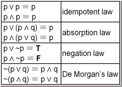
Here are some common laws of logic and some notes identities that you should memorize:

True-False Laws
image

image

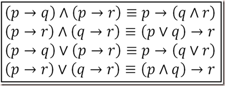
Some laws for implications:

image

Some laws for bi-conditional statements:
image


PREDICATION & QUANTIFICATION

Sometimes, we can use predicates to represent a logic statement, which depends on an unknown, or various unknowns. A predicate is normally denoted by P(x), or any capital letter followed by a bracket with an unknown in it. For example, C(x) may represent “x is a comedian” while F(x) may represent “x is funny”.

A quantifier is used to generalise or specialize a particular predicate, and is placed in front of it. There are 2 kinds of quantifiers:

1. The universal quantifier, denoted by ∀xP(x) which means ‘for all x, P(x)’. It also could mean ‘for every’, ‘all of’, ‘for each’, ‘given any’, ‘for arbitrary’ or ‘for any’. In terms of P(x), it can be represented by the logical statement
image
which means the conjunction of any variable in the predicate P. Using the example above, if x means ‘people’, then ∀xC(x) means ‘everyone is a comedian’.

2. The existential quantifier, denoted by ∃xP(x) which means ‘for some x, P(x)’. It also could mean ‘at least one’, ‘there is a…’ or ’there exists’. In terms of P(x), it can be represented by the logical statement
image
which means that it is the disjunction of any variable in the predicate P. Again, using the example above, ƎxC(x) means ‘some people are comedians’. Sometimes, you might also see the expression Ǝ!xC(x). Instead of ‘for some x’, this means ‘there is exactly one x’. We call it the uniqueness quantifier.


We use these quantifiers just the same way how we use those p’s and q’s earlier on, you can add the negating sign (~) or the conditional arrows (↔ and →) to them. So what are the truth values of these quantifiers?

The statement ∀xP(x) is TRUE if P(x) is true for all x, in which x should belong to a particular domain (people, animal, students or etc). It is FALSE if we could find an x in which P(x) is false. Using the same example again, ∀xC(x) is true if every human being is a comedian, but is false if you could find one person (yes, you only need one person) who isn’t a comedian.

The statement ƎxP(x) is TRUE if there exist one x which is true, and is FALSE if every x is false for P(x). Using the same example, ƎxC(x) is true if there is one human being on earth is a comedian, but is false if you can’t find a single human being who is a comedian.

Simple? Let me give you some common rules for quantifiers:
image

This one tells you how you can bring the quantifier into the brackets. Beware though, you can’t bring a universal quantifier in if you use a disjunction, and the same applies to the existential quantifier and conjunctions.

The negations of quantifiers:
image
This is quite straightforward.


A nested quantifier is formed when you use 2 or more quantifiers in 1 predicate. Examples are like

image

Notice that both quantifiers mean different things. The first one says ‘for all x, there exist a y such that P(x,y) is true’, while the second one says ‘there exist an x such that all y is true for P(x,y)’. Let me give you a detail example:
Let P(x,y) be the statement “x has sent an SMS to y”, where the domain of x and y are ‘students’. We can see that

1. ƎxƎyP(x,y) means “There is some student who sent an SMS to some student.”
2. Ǝx∀yP(x,y) means “There is a student who sent an SMS to all other student.”
3. ∀xƎyP(x,y) means “All students sent an SMS to at least one student.”
4. Ǝy∀xP(x,y) means “There is a student who receives an SMS from all students.”
5. ∀yƎxP(x,y) means “Every student has been sent an SMS by at least a student”
6. ∀x∀yP(x,y) means “All students have sent an SMS to all students.”

Notice that ƎxƎy and ƎyƎx do mean the same thing, and this applies to ∀x∀y and ∀y∀x too, but not the mixture of both. Now the problem is: how do you know the truth values for nested quantifiers? I’ll show you in a table below:
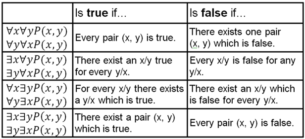
image

You can actually work it out yourself by using the negating rules stated above. It’s simple: a negation sign passes through a universal quantifier turns into an existential quantifier, and vice versa. Another important remark is this:
"if Ǝx∀yP(x,y) is true, then ∀yƎxP(x,y) is true, but not INVERSELY.”


That’s all for logic. You should practice more on translating sentences into logical statements, because it can be very confusing sometimes. Also, practice how to prove the equivalence of logical statements using the given laws. For complicated equivalences (more than 2 propositions), you could use a truth table. It will be faster. We’ll start doing proofs in the next section.

Tuesday, May 24, 2011

SYLLABUS

So what is covered in the Further Mathematics T 1993-2012 syllabus?

In paper 1, you will be learning mostly extensions of what you learn in Maths T. Of course, this will be the harder paper of the two:

1. Logic & Proof
Still remember all those p q stuff that you learn in SPM Mathematics? Logic is a study of propositions, statements which are either true or false. One needs logic to deduce many Mathematical results. You need to know what are conjunctions (and), disjunctions (or), implications, equivalence relations, what is a converse, inverse and a contrapositive of a proposition. There are some other terminologies like tautology, contradiction or counter-example which you will eventually learn what they are. Then you will learn predicates and quantifiers, which are used to generalize (all x) or specialize (some x) the propositions that you came up with. Then in the next section, you will be studying essential methods of proofs which will help you proof some laws or formulas. Examples of proofs are direct, indirect proofs, proof by contraposition, proof by contradiction and etc. Lastly, you will learn the most important proof, which is Mathematical Induction.

2. Complex Numbers
In Maths T, you will learn the basic operations for complex numbers in the Cartesian form. In FMT, you will be focusing on its polar form, and you will learn quite a lot of geometrical significance of complex numbers. You will learn how to prove and use the applications of the famous de Moivre's theorem, which will be something new to you! After studying this chapter, you will be able to solve difficult equations involving complex numbers, or rather use complex number methods to solve some problems. The hardest part of this chapter, I think, is still learning how to illustrate complex number equations as loci in the Argand diagram.

3. Matrices
After learning matrices in Maths T, you thought that matrices is the easiest thing to score. Coming to FMT, you are wrong. Still continuing to use those 3 × 3 matrices, you are going to learn how powerful matrices can be in solving linear algebra! You will eventually find out that not all systems of equations have solutions, or rather, how to know whether they have a unique, infinitely many or no solution. You will be focusing a lot on determinants and their operations, which you touch only a little in Maths T. Then, you will learn how to use Gaussian elimination, Cramer's rule and Cayley-Hamilton theorem to solve and play around with systems of equations of 3 unknowns. In the end, you will learn how to find eigenvalues and eigenvectors of a 3 × 3 matrix, and their significance.

4, Recurrence Relations
This chapter is one of the hardest, partly because the resources on this topic is hard to find, and also a lot of understanding is required. To fully understand this chapter, prior knowledge of Sequence and Series from Maths T is required, and mastering the chapter Differential Equations later on will help too. You will get to understand what does 'recurrence' mean, learn how to find general and particular solutions for recurrence relations equations. The toughest part for you in this chapter is to learn how to solve problems that are modelled by recurrence relations.

5. Functions
This chapter really has nothing much to do with the one in Maths T. Instead, this chapter focuses on the analysis and solving of 3 kinds of functions, namely the inverse trigonometric (sin-1, cos-1, tan-1), hyperbolic (sinh, cosh, tanh) and also the inverse hyperbolic (sinh-1, cosh-1, tanh-1) functions. At last, you get to understand what is that sinh thing in your calculator! This chapter will focus a lot on memorizing of formulas (tonnes of them), proving them, sketching their graphs and solve equations which comprises of these functions.

6. Differentiation and Integration
As if differentiation and integration in Maths T wasn't enough, you will be bombarded with a whole new set of differentiation and integration formulas. You take one step further from Maths T to learn how to determine the differentiability of a function, as well as to find the second derivative of a parametric and an implicit function. You will be learning how to differentiate and integrate those nasty functions stated in the previous chapter, as well as learning how to use them in substitution. You will learn about the reduction formulae of certain definite integrals, normally learning how to prove them. In addition to the evaluation of area under the curve and the volume of revolution you learned in Maths T, you will now learn how to find the arc length and the surface area of revolution. Scary right? This is hard core calculus man….

7. Power Series
Not Power Rangers Series. This chapter will answer your doubt in Maths T paper 2, the place where you saw the proof for the Poisson Distribution. This chapter will is a continuation of the Series that you learn in Maths T, and it will introduce to you that every function can be written in the form of a series, which can be either a Taylor or a Maclaurin series (You will learn Fourier and Laplace in university). You will learn how to use the remainder theorem to approximate some functions. A lot of differentiation and integration will be used in this chapter. L' Hôpital's rule and D'Alembert's ratio test are 2 other concepts you will learn here.

8. Differential Equations
Probably the easiest chapter in the whole of Paper 1. After learning this chapter, you will say that the differential equations you learn in Maths T is really NOTHING at all. You now learn how to solve first order linear differential equations by using an integrating factor. Then you will progress to solve 2nd order linear differential equations, finding the complementary function and particular integral, and thus find the general or particular solution. The good thing about this chapter is that there is not much problems they can model for you in the exam, the questions will be more straightforward.

In paper 2, you will be learning a whole new set of chapters. You will learn 2 basic theories from discrete mathematics, 2 chapters of advanced geometry and 4 chapters of statistics. This is definitely the easier paper:

9. Number Theory
Number theory, as most people say, is the "Queen of Mathematics". It is probably the hardest chapter to score, not only because there is little low-level resources about it, also because it is hard to understand. You will be learning about divisibility of numbers, and you never knew it could be that hard! Understanding prime and composite numbers, finding greatest common divisors (gcd) and least common multiples (lcm), which you have learned in form 1 (probably you have forgotten about it totally)! Then, you will get into detail analysis to study some theorems and algorithms, and the main part will be the study of modulo congruences, stuff like a ≡ b (mod m). This is one tough chapter, and normally ignored by most people because it's hard and only comprises of a few marks.

10. Graph Theory
Bar graphs? Line graphs? No way! Graph theory has nothing to do with all those statistical graphs that you learnt in Maths T. This is one chapter that you will be doing a lot of drawing. You will learn what exactly a "graph" is, and a lot of its related terminologies. vertices, edges, walks, paths, cycles, circuits and etc. You will be exposed to Eulerian and Hamiltonian paths and learn how to identify or solve problems modeled by them. You will also learn how to use Matrix to represent graphs. Interesting right? It can be one of the easiest chapters in this paper when you fully understand it.


11. Transformation Geometry
When you learned transformation in form 4, you only learned them qualitatively. Here in FMT, you will be dealing with matrices, and how to use them to represent a transformation in 2 dimensions (only). Rotations, translations, reflections, scaling, and you will be introduced to 2 new transformations: stretching and shearing. It is good to study matrices in Maths T before you start this chapter.

12. Coordinate Geometry
In Maths T, you stop only at 2 dimensions. In FMT, you will be doing coordinate geometry in 3D, which is not only hard to visualize, but also hard to solve them. You will find out that a line can be represented by various forms, and the equations of lines are not unique at all! In 3D, you will learn about planes and how to represent them, but not solids (thank goodness). Then you will be taught how to find the intersections, angles, or shortest distances between lines, planes or both. This part is really challenging, but will be easy if you manage to memorize all the formulas.

13. Sampling & Estimation
If you would have noticed, this is the very same chapter that appeared in Maths S paper 2. Yes, this is the starting of the 4 chapters of statistics, which are the easiest parts of the paper! In real life, we need to do some surveys and samplings in order to evaluate our business, or maybe to improve the service of a newly started company. You will learn to differentiate what is a population and a random sample, and using the sampling distributions to solve problems. You will use the central limit theorem to make samples of large sizes easier to evaluate. Other than the Binomial, Poisson and Normal distributions, you will learn a new distribution called t-distribution and when to use it. This chapter will then focus more on confidence intervals, how to obtain them and interpret them based on a large sample, small sample or a population proportion. You can study this chapter immediately after doing chapter 5 in Maths T.

14. Hypothesis Testing
No, this is not Physics or Chemistry experiments. You need to test a hypothesis, which is normally a 'claim' by a company regarding their products or services, in order to know whether they are genuine, or liars. You will learn how to formulate a null and alternative hypotheses, use a systematic way to test them using different distributions you learned earlier on based on different situations. You will learn how to determine and identify critical regions based on what significance level you use, in order to decide whether to reject or accept the null hypothesis. You will also learn some concepts like type I and type II errors, and how to use or find them.

15.
χ2 Tests
It's not x2, it is "chi-squared' tests (chi, read as 'kye' is a greek alphabet).
χ2 tests are used to determine whether a sample belongs to a certain distribution. The method of doing it is very similar to hypothesis testing, but much easier. You will learn how to use χ
2 tests to determine goodness of fit or independence in a contingency table. It is quite a straightforward and short chapter, don't worry.

16. Correlation & Regression
This chapter also appears in paper 2 of Maths S. This is what I called as 'hard-core statistics'. This chapter will teach you how to make use of the full power of the statistic functions in your calculator! You will first learn about scatter diagrams. Using these scatter diagrams, you will then learn about the concept of correlation, interpret the Pearson correlation coefficient, and then the drawing of regression lines. In the end, you will learn how to use the relationships between correlation coefficient, regression coefficient and the coefficient of determination. This chapter can be very messy in calculations, so as I said earlier on, your calculator will be really useful here. This is also the only chapter whereby you might possibly need a graph paper.


If you are reading through this before you even started STPM, don't be scared by the terminologies. You must have the craving to understand everything. You can start spending time to Google about these stuff when you are free. There is still a lot to learn about Mathematics later on. As you can see, paper 2 is half statistics, half hard core mathematics. The strategy of this paper is to do perfectly in the statistics, and do your best for the rest. Not hard to get an A if you put enough effort into it. Note that I will giving you lectures on all the 16 chapters. What I will do is I will upload some tips or short notes for you to prepare for the exam. You are still required to study the textbooks and spend time understanding them.

Friday, May 20, 2011

INTRODUCTION

What is Further Mathematics T?

Further Mathematics T, as it names suggests, was an extension of the Mathematics T subject used for the STPM syllabus of 1993-2012. It was, of course, harder than the original paper, covers another 16 more topics, and is beneficial for those who are thinking of pursuing their studies in the fields of Physics, Mathematics, Engineering, or any mathematical related courses. Further Mathematics T was to be taken as the student’s 5th STPM subject (the maximum amount of subjects you can take is 5 in STPM), but it must be taken with Mathematics T. The most common combination of subjects for Further Maths candidates are Pengajian Am, Chemistry, Physics, Maths T and Further Maths T.

Further Mathematics T was not an easy paper. In fact, it is the hardest paper, and there are very few candidates taking it every year. Let me show you some statistics:

2008 – 36 candidates

2009 – 16 candidates (only 2 candidates passed. I was the only 'calon sekolah kerajaan'!)
2010 – 22 candidates

(source: taken from MPM website every year)

From the figures, you can guess that you can rarely find a Further Mathematics T teacher out there. Certain schools in Penang and Ipoh might have teachers teaching in school, but not in any other of the 12 states in Malaysia. Further Mathematics T candidates basically study independently, and have to do a lot of self studies in order to score a decent grade for it.

Do you want to take Further Mathematics as your 5th STPM subject? This blog may be a little out-dated, as the syllabus has been changed in 2012, but it still contains certain chapters which are still relevant for you. Feel free to browse through, I am here to assist those who are willing to challenge themselves to the hardest.