Before I continue, I need to teach you some basics of transformation. You will learn the further details in Chapter 11.
You probably still remembered the transformations you learnt in form 4 Mathematics. There are translations, enlargement, rotation, reflection and etc. Basically, every kind of transformation, whether in 2 dimensions or 3 dimensions, can be represented by a matrix. I won’t be teaching you how, but you need to know this before I continue. So it simply means that a vector (x, y), after being transformed by the transformation T (which can be represented by a matrix) will change its coordinates to (x1, y1). It can be written as
Now, in some special cases, you will find that a particular line after undergoing transformation T, will remain unchanged. A good example is the reflection across the line y=x. You can reflect the line y = 2x and it turns into the line 2y = x. However, you find that the line y = x, after the reflection, is still y = x! This line is called an invariant line.
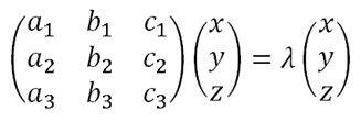
An eigenvector is a vector pointing in the direction of an invariant line under a particular transformation. An eigenvector is not unique, for example, the eigenvector for the line y = x could be (1, 1), (2, 2) or etc., but they both mean the same thing. An eigenvector, after the transformation T, will still fall in the same line (same direction, or rather, same ratio between x and y), but not necessarily the same position. So using matrices, we can represent the transformation T as
Notice the right hand side. Since I said earlier that the vector (x, y) after being transformed, will still be in the same line (same x:y ratio), it means that it will just transform to another vector (x, y) multiplied by a constant λ. λ is what we called as an eigenvalue.
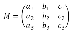
The aim of this section is simple, you just need to know how to identify the eigenvalues and eigenvectors. I’ll be focusing on 3D vectors in this section (you will learn them in detail in Chapter 12). So let’s say we let the transformation M be
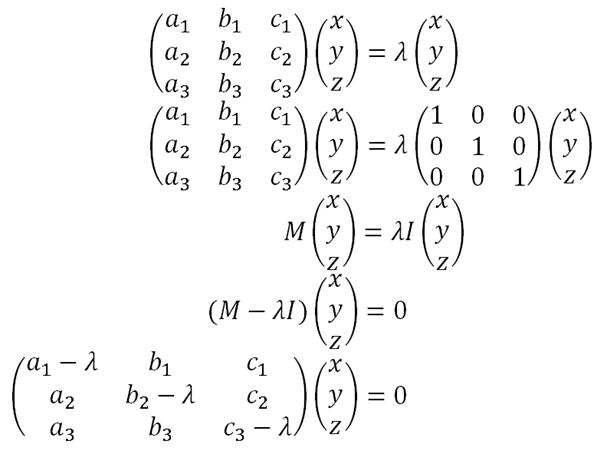
As I said, our aim is to find what is the eigenvector and eigenvalue for this transformation. Let’s try to find λ. Doing a little algebra,
Now let’s get back to determinants. Looking at the situation, we know that the determinant of the big chunk matrix over there must be zero, because since the eigenvectors are not unique and are non-zero. Besides, there’s no particular x, y or z that we are finding, it is an invariant line, which is dependent on a parameter t (recall your coordinate geometry in Maths T). So we are almost there! By writing down
we can find λ by forming a quadric equation, then we can substitute it back to the initial equation to find its eigenvector. Let me show you an example:
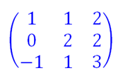
FInd the eigenvalues and their respective eigenvectors for the matrix
So let’s start by finding the eigenvalues.
(1 - λ)[(2 - λ)(3 - λ) - 2] – 1(2) + 2(2 – λ) = 0
λ3 – 6λ2 + 11λ – 6 = 0 [this equation is called the characteristic polynomial]
λ = 1, 2, 3
So by simplifying the equation and using your calculator, you find that this matrix has 3 eigenvalues. Note that it is possible such that a matrix only has 2, 1, or no eigenvalues. Now that we found the eigenvalues, let’s try to find the eigenvectors. We need to substitute each value of into the equation
When λ = 1,
We get a system of linear equations,
y – 2z = 0
y – 2z = 0
-x + y –2z = 0
So you immediately notice that this is actually a system of linear equations which are linearly dependent. Letting z = t, you have (x, y, z) = (0, –2t, t). However, your answer is not .
.
as you need to substitute a value for t into it. So your answer should be (0, –2, 1). Note that you can also put (0, –4, 2), (0, –2.666, 1.333) as any scalar multiple of any eigenvector is still the same eigenvector. But we really chose the first one for simplicity.
Hey, the working is not done yet!
When λ = 2,
…
…
the eigenvector is (1, 1, 0)
When λ = 3,
…
…
the eigenvector is (2, 2, 1)
Try do the working yourself.
In the end, you find yourself with 3 eigenvalues and their respective 3 eigenvectors. The finding process may be hard if you are a careless person. So please do a lot of practices on this section.
CAYLEY-HAMILTON THEOREM
If the characteristic polynomial p(λ) of an n × n matrix A is written
p(λ) = (-1)n (λn + bn-1λn-1 + … + b1λ + b0), then
An + bn-1An-1 + … + b1A + b0I = 0
Basically what this theorem means is that the λ in the characteristic equation of the matrix can be substituted with the whole matrix itself. Taking the characteristic equation example above,
λ3 – 6λ2 + 11λ – 6 = 0
tells us that actually
M3 – 6M2 + 11M – 6I = 0
where M is the matrix itself.
From here, you could actually find the inverse matrix M-1 a fast way. Post-multiplying M-1 to the equation, we get
M2 – 6M + 11I – 6M-1 = 0
and from here we will get

That is the only reason I think Cayley-Hamilton Theorem is used for.
This chapter should end here. However, I think it is better that you know some applications of eigenvalues and eigenvectors. One such application is diagonalization.
DIAGONALIZATION
We can actually represent a matrix in terms of its eigenvalues and eigenvectors. Taking the blue example above, first, let’s represent all its eigenvalues in terms of a diagonal matrix (try recalling what a diagonal matrix is).
Notice that 1, 2 and 3 are the eigenvalues of M in the example above, and that they only occupy the diagonal of the matrix. This matrix shall be denoted as D. Next, squeeze their respective eigenvectors together (in the correct order), and we find its inverse. This matrix here, we shall call it P. 
From here, you will be able come out with the results such that
D = P-1MP
But this is not the result I want. Post multiplying with P-1 and pre multiplying with P, gives us
M = PDP-1
This result is very important, especially when we want to raise the matrix M to a certain power. For example,
M2 = PDP-1PDP-1 = PD2P-1
The exponent of a diagonal matrix is very straightforward, as in
So this is one of the very fast ways you can find the power of a certain matrix. If you have time, you should try to verify that M = PDPT holds if M is a symmetric matrix (PT denotes the transpose of P), and also if the eigenvectors in P are normalised, that means, the eigenvectors are unit vectors (or rather, your chosen form of eigenvector (x, y, z) divided by
√(x2+y2+z2)).
That’s it for this chapter. Go and tell your high school classmates and brag to them about eigenvalues and eigenvectors that you learn here. ☺

No comments:
Post a Comment